Splitting text on white-space efficiently in Java

Small data, small problem. Big data, ...

Splitting text on white-space in most programming languages is normally a trivial matter. This task becomes a lot more difficult though when you try to complete it over a very large document collection.

The easiest way to split a document on white-space is to use the split method, which is implemented by default in most languages on String objects. Although the split method produces the end result we are looking for, it is not the most efficient way to manipulate large sets of data.

Strings and Streams

In Java, it can be advantageous to use streams over Strings since streams allow the programmer greater flexibility in the specifying the I/O buffer size. By specifying an optimal buffer size for the input stream, the programmer can reduce the the number of disk reads that need to be performed in order to load the contents of a file into memory. Less I/O means more performance.

Use Buffered I/O (for text documents, in this case)

Since the purpose of buffered I/O is to reduce the number of disk reads necessary to load a file, you can imagine that knowing the size of the file prior to loading it is important. After the size of the file we want to load is known, we create a character array store the contents of the file one character at a time. (Note that the character encoding of the document you are reading impacts the number of bits or bytes used to represent a character.)

The Split Function

At this point we have our document stored within a char array and need to start splitting it into individual words or tokens efficiently. Since we are dealing with a char array, we no longer have the String method "split" available. The strategy here is to step through the entire char array (document) one time and pick out all of the words to be stored (say in a dictionary). In order to achieve this task the trick is to keep track of when a word begins and ends in the stream. This can be done by using a simple Boolean flag within the loop which iterates through the character array.

First determine whether or not the first character is white-space or not. This is important since we need to know whether we are looking for the beginning of a word first or whether we're looking for the end. Assuming the document starts with a word instead of white space, we take note of the fact that we are currently iterating over a word. Once we realize that the word has ended (a space has been encountered) we mark the end of the word, add it to the dictionary and set our Boolean flag to record that we are no longer on a word. At this point, as we iterate through the document further, should any additional white-space be encountered, it will be ignored. The next time something interesting happens in the code is when we reach a non white-space character, at which point we reset our Boolean flag to reflect that we are at a word boundary again and take note of where it starts. Then we move on looking for the next instance of white-space to find the ending boundary of the latest term discovered.

I know that explaining an algorithm can often sound convoluted and so I have attached a small code sample that demonstrates the technique of using streams and character arrays to efficiently process large document sets.

import java.io.File;
import java.io.FileInputStream;
import java.io.FileNotFoundException;
import java.io.IOException;
import java.io.InputStreamReader;
import java.io.Reader;
import java.io.BufferedReader;
import java.util.ArrayList;

public class Driver {

	public static void main(String[] args) {
		// Set the location of the corpus
		File corpus = new File("/path/to/document/collection");
		// Iterate through the files and perform the necessary actions
		File[] files = corpus.listFiles();
		for(File f : files) {
			try {
				
				// Get the size of the file, create a byte stream and a character array to store the input
				int file_size = (int) f.length();
				Reader input = new BufferedReader(new InputStreamReader(new FileInputStream(f)));
				char[] data = new char[file_size];
				
				// Create an array list to store the tokens
				ArrayList tokens = new ArrayList();

				// Read the file
				while (input.read(data, 0, file_size) != -1) {

				  // Determine whether we are starting with whitespace
				  boolean at_token = Character.isWhitespace(data[0]) ? false: true;
				  
				  // Keep track of the bounds of tokens
				  int left = 0, right = 0;
				  
				  // Iterate through the data stream
                  for(int i = 0; i < data.length; i++) {
                	// Found the beginning of a token
                	if (!Character.isWhitespace(data[i]) && at_token == false) {
                      at_token = true;
                      left = i;
                    }
                	// Found the end of a token
                	if (Character.isWhitespace(data[i]) && at_token == true) {	
                      at_token = false;
                      right = i;
                      StringBuilder token = new StringBuilder(right-left);
  					  token.append(data, left, right-left);
  					  tokens.add(token.toString());
                    }
                  }
				}
				int ctr = 0;
				for (String s : tokens) {
					System.out.println("Token #"+ctr+"\t"+s);
					ctr++;
				}
			} catch (FileNotFoundException e) {
				e.printStackTrace();
			}
			catch (IOException e) {
				e.printStackTrace();
			}
		}
	}
}

Starting a new Repository on GitHub

These are the instructions that GitHub provides you with in order to create a new repository.

Note: replace the name John Doe with your actual GitHub user name. Also replace the email and don't forget to name your app.

Global setup:

Download and install Git
  git config --global user.name "John Doe"
  git config --global user.email john.doe@gmail.com
        

Next steps:

mkdir Name-Your-App
  cd Name-Your-App
  git init
  touch README
  git add README
  git commit -m 'first commit'
  git remote add origin git@github.com:JohnDoe/Name-Your-App.git
  git push -u origin master
      

Existing Git Repo?

cd existing_git_repo
  git remote add origin git@github.com:JohnDoe/Twitter-Apps.git
  git push -u origin master

Git Handbook

Git is version control software that allows coders to tinker with their code without compromising the project's code. Here are the basics you'll need to git going with Git.

---

Git Configuration
Set your email that will appear in commit messages.

git config user.email youremail@example.com

Set your name that will appear in commit messages.

git config user.name 'FirstName LastName'

Recommended: Tells git-branch and git-checkout to setup new branches so that git-pull will appropriately merge from that remote branch. Without this, you will have to add --track to your branch command or manually merge remote tracking branches with "fetch" and then "merge".

git config branch.autosetupmerge true

You can add "--global" after "git config" to any of the above commands to make it
apply to all git repos (note this will edit the ~/.gitconfig).

Clone the specified repository by <repo> this is similar to "checkout" in some other version control systems such as Subversion and CVS

git clone <repo>

---

Gathering information from Git

git diff

Show files added to the index, files with changes, and untracked files

git status

Show recent commits, most recent on top

git log

Show the changeset (diff) of a commit specified by <rev>, which can be any SHA1 commit ID, branch name, or tag

git show <rev>

Show who authored each line in <file>

git blame <file> 

Show who authored each line in <file> as of <rev> (allows blame to go back in time)

git blame <file> <rev>

---

As usual,  you can expect more to come soon.

Software Architecture

Definition of Software Architecture (IEEE 1471-2000)
The fundamental organization of a system [as] embodied in its components, their relationships to each other, and to the environment, and the principles guiding its design and evolution.


Where does software architecture fit in?

Rational Unified Process (RUP)

Software architecture becomes increasingly important as the size of the code base and project increases. This doesn't mean that you should neglect the architecture of a project until it becomes too difficult to manage. In the context of the Rational Unified Process (RUP), the architecture would be considered between the requirements and implementation phases, effectively during the analysis and design stage. In terms of the design, the architecture can be viewed as the top-level design which is then further elaborated upon in the detailed design (Class diagrams, System Sequence diagrams, etc...). Naturally, since the architecture can be viewed as the top-level design, and fits into the RUP just after the requirements phase has commenced, a highly dependent relationship exists between the two phases. As we've seen above, architecture can be viewed as a form of design, but it should be noted that not all design activities are architectural activities. The levels of  design, from the top-most layer are, architectural design, detailed design and lastly the implementation (executable designs).

Benefits of an Architectural Design
- Reduced rates of failure
- Qualify rationale for architectural decisions
- Outline and mitigate risks
- Schedule and cost projects more effectively
- Useful for learning about the system
- Re-use of architectural styles
- Increases maintainability

Requirements Versus Design

Requirements Artifacts	Design Artifacts
Domain Model	Software Architecture Document
Use-Cases	Design Model
Non-Functional Requirements	User-Interface Design

How To Start Your Design
A natural way to begin the design is to build on some of the work that you've already put in. The domain model is an excellent place to create the first approximation of the design  as it guides the designers into crafting a solution with a minimal representational gap. Whenever tasked with creating a design for a software project always consider whether this same type of application has been created in the past. If so, then analyze how the current solutions are implemented and make use of whatever code or structure is available. Quite often an architectural style will have already been applied to the problem which you may likely want to re-use.

Common Architectural Styles
Data-Flow	Data-Centered	Virtual Machine	Call and Return	Independent Components
Pipes and Filters	Repository	Interpreter	Main Program and Subroutine	Communicating Processes
Batch Sequential	Blackboard	Rule-Based System	Object-Oriented (& Data Abstraction)	Client/Server
			Layered	Event Systems
				Implicit Invocation
				Explicit Invocation

Conceptual Integrity
"I will contend that Conceptual Integrity is the most important consideration in system design. It is better to have a system omit certain anomalous features and improvements, but to reflect one set of design ideas, than to have one that contains many good but independent and uncoordinated ideas."

- The Mythical Man-Month, by Fred Brooks, 1975


Enterprise Applications
Generally, enterprise applications form a class of software solutions that deal with large volumes of complex data that is persistent and concurrently accessed by many users and or applications. The software does not usually have strong hardware/software integration requirements. A common approach to constructing enterprise applications is to use the layered or client-server architecture.


Enterprise Application Architectural Styles
As we've just seen, two very common architectures are often employed in the construction of enterprise applications. We'll now take a closer look at both styles.

Layered Architecture
At the most basic level, the layered approach typically consists of at least three layers: presentation,  domain and data source. As far as functionality is concerned in the this architecture, lower level layers service requests from higher ones, thus providing functionality upwards from the bottom. Dependencies however move in the opposite direction from higher level layers to lower ones. One variation of the classic layered style exists, the pure layered style, where the dependencies are further restricted by allowing higher level layers to depend solely on services from components within the same layer or the layer immediately below.

Presentation 

------------------------------

Domain

------------------------------

Data Source

Client-Server Architecture
Client server applications, such as a web browser will usually utilize the Internet for communications. We'll provide a few quick definitions of what exactly we mean when we say the Internet versus the web. The Internet is the hardware infrastructure in which the web operates. The web is just software along with a set of associated protocols. As an example, Hyper-Text Transport Protocol (HTTP) is a stateless and fairly simple request-response protocol that is used extensively on the web. Now that the Lingua Franca has been defined we can better understand the interaction between the clients and servers. A client is responsible for sending HTTP requests to severs, while servers have the task of sending HTTP responses. A web server is a piece of software which implements the web protocols (i.e. HTTP). The clients (more software) make requests using the web protocol to the web servers and receive responses. Web servers can only serve static content, thus helper applications are needed in order for the server to serve dynamic content. An example of one such helper is a Java Servlet. The typical environment in which Java servlets reside is Tomcat, a servlet container. In the weakest possible terms the role of Tomcat is to facilitate the interaction between the web sever and the servlets. Tomcat

HTTP Methods	Description
GET	get a resource a given URL
POST	basically a GET with extra parameters
HEAD	GET the header part of the response only
TRACE	loopback request message
PUT	put info at given URL
DELETE	delete the given URL
OPTIONS	list the HTTP methods the URL can respond to
CONNECT	This specification reserves the method name CONNECT for use with a proxy that can dynamically switch to being a tunnel (e.g. SSL tunneling [44]).

The anatomy of an HTTP request, picture by Dr. Chalin

The anatomy of an HTTP response, Dr. Chalin

Pipes and Filters
The metaphor of pipes and filters can be directly applied as a software architectural style. A pipe carries a fluid through it until it reaches a filter. The filter then outputs it's modified fluid back into another pipe. In using this metaphor  as a basis for the software implementation say that a pipe should carry data between filters and a filter should accept data and output it to a pipe. The advantages of using this data flow style is that it assumes concurrent processing since output from a pipe can be continuously consumed by a filter while simultaneously outputting it's content to another pipe and ultimately filter. Each filters is independent all other filters, thus each filter maintains it's own state. Filters are thought of black boxes and are only responsible for accepting input in a specific format and outputting data in a specific format, thus filters can be swapped easily. No complex interactions exists in pipes, simple data transfers are the only responsibility of pipes. Some weaknesses of this style are that it's use can lead to batch sequential programming, it is also not well suited for interactive applications. As mentioned a data format must be defined for the input and output of the filters, thus additionally complexity is added to the filters for the encoding of decoding of outputs.

Variations of Pipes and Filters
Pipeline: A linear sequence of filters.
Batch Sequential System: A pipeline in which each filter runs to completion before the next begins.
Bounded Pipes: Restriction on the amount of data that can be temporarily in a pipe.
Types Pipes: The data passed between two filters is restricted to a well-defined type.
UI Pipes: Each filter is associated with a user-interface to allow the user to set parameters of operation.


Event-Based Architecture
Event-based programming is the chief architecture used in the development of graphical user interfaces. Someone clicks a button for instance and an event is fired notifying someone else that the button has been pressed and action must now be taken. It is also well suited for multi-core systems since events can be processed in a number of locations. UML2 has even made provisions for it within it's specification.

Components and Connectors
A component is an active or passive object, capsule or module. A connector is a callback, channel or binding. Notable component types are publishers and subscribers. A component does not explicitly invoke another component, instead an event is generated (message is passed). In order for a component to become aware of events stemming from another component it must subscribe or register with component. This relationship can be thought of as subscribing to a newsletter for instance. I must register myself on the subscribers list in order to be notified of updates. Once I am notified I can take whatever action I choose, read, disregard, forward, etc... A connector is tasked with carrying events being signals or messages from one component to another. Connectors can have a range of multiplicities with components, ranging from one-to-one to one-to-many, or many-to-one. The advantage of using this style is that it encourages code reuse through low coupling and provides opportunities for evolution as new components are introduced. Asynchronous communication is handled extremely well within this type of design. All of the weaknesses that arise in this architectural style stem from the lack of control components have over event processing. Components are restricted to simply generating events while a framework is tasked with the event dispatching. Furthermore, respondents to events are not ordered, sometimes making global system analysis more challenging. Asynchronous events explicitly highlight this problem. ow can we ensure that at least one object has processed an event? Another weakness associated with this style is a problem arising from the exchange of data between components which can lead to a resources management challenge.

Process Control
This architectural style is particularly well suited for modeling physical control systems. In this model software interacts with peripheral devices like sensors and actuators in order to control physical systems. This architecture can be applied in real-time, continuous, adaptable (load balancing) and control system environments. The disadvantages of this architectural style are that the reuse of components are often confined to one particular domain of the application and it can become difficult to adapt when are two or more interdependent processes to control.


Architectural Views

4+1 View Model

When analyzing the architecture of a system it is often most useful to consider the aspects of it relative to a particular view. A view is a fairly intuitive term in terms are architecture, it implies looking at something from a specific view-point. Naturally a single view-point cannot provide anyone with a complete picture, unless it is one dimensional, which large software projects are not.

"4 + 1" View Model of Architecture
This is one of the most popular view models conceived for software projects by Phillipe Kruchten in 1995.

View	Description	Artifacts
Logical View	The logical view is where the overall structure of the application is conveyed. Another way to characterize the logical view is to think of it as the interfaces to the environment in the most general of contexts.	- Package Diagrams - Class Diagrams - State Diagrams - Interaction Diagrams
Process View	The process view is used to paint a picture describing the underlying processes and tasks which are occurring within the system, as well as the channels of communication between them. The interrelationships amongst processes should be visible as well as the synchronization mechanisms.	- Class Diagrams - State Diagrams - Interaction Diagrams - Component Diagrams
Deployment View	The deployment view, sometimes called the physical view, is used to describe the hardware and software setup that is required by the system. In this view we gain an appreciation of how the hardware and software components are combined to form the deployed product.	- Deployment Diagrams
Implementation View	The implementation view, sometimes called the development view, provides perspective on the software's organization. The components of the system as well as their inter-dependencies are outlined within this view. Libraries, sub-systems, executables, object files, etc. are all commonly documented components in this view. The relationships are denoted through containment and dependencies, thus providing a high-level vantage point for observing the software's organization.	- Package Diagrams
Use Case View	The use case view takes it's place prominently in the middle of the above 4+1 view model diagram, and rightfully so. It is the use cases which necessitated the system in the first place thus any model would be incomplete without it's raison d'être. Each system is designed to satisfy the needs of some target user, and the use case view elaborates on the systems utility from the users perspective. Note that not all use cases will be represented here, only those with the most architectural significance.	- Use Case Diagrams

Siemens Four View Model
This view model prescribes activities that should be carried out within each view. The activities are, global analysis, central analysis and final analysis.

Global Analysis
1) Analyze factors
2) Identify Issues
3) Create Strategies

The purpose of global analysis is to identify issues early in the architecture so that strategies can be proposed to resolve them. Factors are further decomposed into the following three categories: Product, Organizational, Technological. Issues simply implies a potential problem or risk. Strategies alludes to a means by which an issue is resolved.

Organizational factors can be further decomposed into the following top level groupings:
management, staff skills, process and development environment, development schedule and finally the development budget.

Product factors are:
Functional features, user interface, performance, dependability, failure detection (reporting and recovery), service and product cost.

Design Principles
Definition of a good design: A good design satisfies all of the requirements and passes all tests. It is also as simple as possible and conveys intent. There is no duplication and it's easy to understand, verify, extend and evolve.

Fundamental software design principles:
- Information hiding (Parnas)
- Protected Variations (Larman)
- Open-Closed Principle (Meyer)
- Separation of Concerns (Dijkstra, Parnas)
- High cohesion (GRASP)
- Low coupling (GRASP)

Object Oriented Design Principles
Design based on responsibility assignment
- GRASP (Larman)
- Responsibility-Driven Design, RDD (Wirfs-Brock et. al.)
- Class-Responsibility Collaboration Card Design Technique (Kent Beck, Ward Cunningham)

General Responsibility Assignment Principles (GRASP)

Controller

Creator

Indirection

Information Expert

High Cohesion

Low Coupling

Pure Fabrication

Protected Variations

Polymorphism

Software Design Patterns
GoF Design Patterns

Behavioral Patterns	Creational Patterns	Structural Patterns
Chain of responsibility	Abstract Factory	Adapter
Command	Builder	Bridge
Interpreter	Factory Method	Composite
Iterator	Prototype	Decorator
Mediator	Singleton	Facade
Memento		Flyweight
Observer		Proxy
State
Strategy
Template Method
Visitor

Data Source Software Design Patterns

Row Data Gateway (RDG)

Table Data Gateway (TDG)

Active Record

Data Mapper

Document Object Model (DOM)
The document object model describes the structure of a document in a hierarchical context. Consider an HTML page, it is organized as a tree of tags, where the first tag is <html> and last tag is </html>. Thus this tag is the root of the tree which is then followed by the <head> and <body> tags. More complicated hierarchies of tags arise when we begin to consider cascading style sheets. They allow stylistic hierarchies to be created for web content and stored separately from the content itself, providing a layer of indirection. The tags in an HTML page can be generalized to the concept of nodes of which the following types exist.

DOM Node Types:
- Document
- Element
- Attribute
- Text
- Comment

Architectural Definition Languages
This field is currently under continuous research and has not yet come to reach it's full potential. The concept here is to create a new higher level language that could serve to define both the structure and behavior of a program leading to executable code. I should point out that the scenario of producing executable code has not yet been completely realized. At the moment the best that can usually be done is creating the skeletons of the classes with method and attribute placeholders that would later be filled in. Some applications of code generation however have been quite successful, Boeing reported to have generated 75% of the code that was developed for their new 747. A closely related field is Model Driven Architecture (MDA) and Model Driven Design (MDD). The most notable of players in the market is IBM with it's Rose platform.

There will be more to come on this post... very soon.

Usability Engineering

Overview

Human Computer Interaction and Interaction Design

The goal of usability engineering is to optimize the user experience within your applications. Ideally the customer should be able to interact with your product in a manner that feels most natural to them. This is much easier said than done when considering the diversity of an applications user base, especially as the internet continues to proliferate. In order to maximize the quality of the user experience we will take an in depth look at the various activities that a software engineer should take in order to produce the highest quality application, in terms of user interaction and experience. The diagram on the right shows all of the different disciplines that relate to human computer interaction (HCI). As you can see there are a lot of professionals related to this practice, thus forming a well rounded team with specialists from as many disciplines as possible is a great way to generate good ideas within your team.

Good and Bad Designs
In order to appreciate good designs perhaps it would be helpful to first look at some bad designs. We have all seen bad designs before, the vending machine the scammed you, the remote control that was too complicated to use. Bad designs come along a lot more of then good designs since considerable effort is required to produce a design that is universally praised by a majority of the user base.  Basically a bad design does not lead the user naturally through workflows within the system, causing considerable confusion and frustration. A good design easily allows the user to recognize which actions need to be taken in order to achieve their goals. I would encourage you to see some proof of bad design in everyday life so that you can see for yourself how rampant bad designs are.

Traits of a Good User Interface
- Helps the user quickly build a mental model of the entire system, not just one part.
- Enables the user to easily build a mental model of the application, leading to intuition for the users.
- Feels natural to user making it easy to learn how to use. Removes any surprises that may cause confusion.
- Feels like it's been tailored to the end-user.
- Allows the user to perform tasks efficiently.
- Meets the principal design goals of: usability, catering to different types of users, etc...

The Tangible Benefits of a Good User Interface
- Enhances the users productivity.
- Reduces the learning curve and associated costs.
- Enhances the end-users' satisfaction.
- Improves the quality of the work performed by the users.
- Minimizes the the number of errors related to workflow processes.

Things You Need to Know to be Able to Produce a Good UI Design
Since we are concerned with the performance of the system relative to our end-users, it is only natural that we focus on them. The following list represents traits of our users that can help guide our UI design choices.

- Users profile, behavior, background, skill level, etc...
- The types of tasks that the user needs to perform.
- The context and social environment in which the system will be used.
- The limitations of what is suitable and feasible from a technological perspective.


The Difficulties of Producing a User Interface Design
Diversity amongst the users base as well as plethora of tasks which need to be performed compound to make the job of the UI designer that much more difficult. Additionally, understanding user requirements is not an easy process, as visible through the large number of software project failures. Additionally, when software begins it's lifetime, UI often takes a back seat since it's the last layer on the cake, although this is not recommended from a usability engineering perspective. The final and most decisive hurdle to most companies getting need to overcome in achieving a high quality UI is the cost associated with the process of researching, prototyping and testing.


The Status Quo From a Software Engineers Perspective (Note this is not acceptable)
- Let us design for technology rather than for the end-user needs.
- Flashy graphics and nice colors to make up for bad design.
- Engineers obsess over program logic while users interact with the application visually.
- Users make errors but we don't plan for them.
- Fix UI bugs with documentation
- Lack of time and budget, so improvements get pushed to the next release, perpetually in some cases.

Tips for Understanding Your Users' Needs
- Take into account your users strengths and weaknesses.
- Consider ways to help your users adopt more efficient work flows.
- Take the time to quantify what how to improve the quality of the user experience.
- Ask people what they want, and don't forget to listen to the answers.

"you cannot design the user experience, you can only design for a user experience"

The Interaction Design Process, Briefly

- Identify the needs and requirements for the suer experience.

- Develop alternative designs to meet these goals.

- Build interactive prototypes that can be evaluated.

- Continuously evaluate what is being produced based on the quality of the user experience.

Core Characteristics of Interaction Design

- Users are involved throughout the development process

- Specific usability and user experience goals must be identified, documented and agreed to by all parties.

- The design process occurs iteratively with time alloted for regular prototype evaluations.

Important Terms for Usability Designers
- Visiblity, i.e. making the actions that a user can perform visible to them.
- Affordance, referring to an attribute of an object that allows people know how to use it, i.e. door handles, computer mice, etc...
- Conceptual model, this is a high-level description of how a system is organized and operates.
- Models, a simplification of some aspect of human-computer interaction intended to make it easier for designers to predict and evaluate alternative designs.
- Framework, a set of interrelated concepts and/or a set of specific questions.

Usability Principles (Nielson 2001)
- Visibility of system status
- Mach between system and the real world
- User control and freedom
- Consistency and standards
- Help users recognize, diagnose and recover from errors
- Error prevention
- Recognition rather than recall
- Flexibility and efficiency of use
- Aesthetic and minimalist design
- Help and documentation


Understanding User Interaction
So far we've highlighted the goals of user interaction design, and have seen what makes a good or bad design. We'll now switch our focus a bit towards understanding how to analyze the problem space (user requirements) so that when we do get to the point of designing out solution we will have a better idea of what problem we are trying to solve.

Analyzing the Problem Space
In order to effectively analyze the problem space we need to keep the following questions in mind.
- What do you want to create?
- What are your assumptions?
-  What are your claims?
- Will your solution effectively aid the user in achieving their goals, and how so?

Analyzing the Problem Space Related to Currently Implemented Solutions?
- Are there problems with an existing solution
- Why do you think there are problems within the existing solution?
- How do you think your proposed design ideas can overcome these issues?
- when designing for a new user experience how will the proposed design extend or change current workflows?

Creating a Conceptual Model
As defined above, the conceptual model is the high level design description of how the system will operate. This is extremely important to do at the beginning of the design process since it will help formulate the overall strategy for the solution to be. By establishing a conceptual model a lot of questions that may arise during the design process can be managed with the overall goal in mind allowing the designers to create a more cohesive solution.

Main Components of a Conceptual Model
- Major metaphors and analogies that are used to convey what the solution has been designed for and how it should be used.
- Concepts that users are exposed to in using the product.
- The relationships between the concepts.
- The mappings between the concepts and the user experience the product is designed to support.

Interface Metaphors
Using a metaphors in your design helps foster intuition amongst users. An effective metaphor allows the uses to grasp the underlying conceptual model with ease. It can also be an innovative way to make your application accessible to more users. A good metaphor is designed to be similar to some familiar physical entity, like a desktop. By likening your virtual solution to some physical entity you can allow the users to build their own intuition quickly about how the product performs.

Difficulties in Creating Interface Metaphors (Nielson, 1990)
- Break conventional and cultural rules (i.e. recycle bins on desktops).
- Can constrain designer in the way which they conceptualize the problem space.
- Conflict with design principles.
- Forces users to only understand the system in terms of the metaphor.
- Designer can inadvertently use bas existing designs and transfer the bad parts over.
- Limits the designers' imagination in creating new conceptual models.

Interaction Types (M.I.C.E.)
The following is a categorization of the various interaction types.
- Instructing: Issuing commands using the keyboard, function keys and selecting options from a menu.
- Conversing: Interacting with the system as if having a conversation with it.
- Manipulating: Interacting with objects in a virtual or physical space by manipulating them.
- Exploring: Moving through a virtual environment or space.

Understanding Users
There are two types of cognition according to Norman (1993), experiential and reflective. Experiential cognition is defined as the type of cognitive exercise where a person is mindlessly interacting with his or her environment. Reflective cognition is when  you deliberately think about an issue and make a decision about it. The reason that it is important to make this distinction is because each type of cognitive process requires different levels of technological support. One thing to keep in mind about all of this is that people have been proven to be much better at recognizing things than recalling them. Additionally, certain types of information are easier to recognize than others, such as pictures. This leads us to the concept of recall-directed memory versus recognition-based scanning. Suppose the user of your system was trying to go to a URL that they were recently at. The first attempt of the user is to remember the URL directly and simply type it in to the navigation bar. When this fails the user resorts to scanning his history for the proper URL since he was there just a few days ago. Although scanning takes longer than remembering something directly the end result was ultimately achieved. This shows us that it is important to provide your users with a couple different ways of locating items of interest in order to provide the most enjoyable user experience. A general strategy when  implementing some of these ideas into a UI is to use recognition rather than recall within menus, icons and consistently placed objects.

Theory of Action (Norman 1996)
The following theory is an approximation of the mental process which occurs in each of us when using software. This theory suggests that software should always provide it's users with meaningful responses in order to inform them whether or not their needs and intentions have been met.

Bridging the gulfs of execution and evaluation, Norman 1986

1) Establish a goal
2) Form an intention
3) Specify an action sequence
4) Execute an action
5) Perceive the system state
6) Interpret the state
7) Evaluate the system state with respect to the goals and intentions





Data Gathering Techniques
1) Interviews
     - Structured
     - Semi-structured
     - Unstructured
2) Focus Groups
3) Questionnaires
4) Observation
     - Field
     - Controlled environment

Installing Tomcat In Ubuntu

Quick how to guide for installing Tomcat in Ubuntu


1) make sure that you have the necessary Java SDK's installed. Use the following bash command:
dpkg --get-selections | grep sun-java

You should have the following output:
sun-java6-bin
sun-java6-jdk
sun-java6-jre

If you get no results back then run the following command in the terminal to acquire the needed Java SDK

user@pc:~$sudo apt-get install sun-java6-jdk

2) Now we're ready to download and install Tomcat available at Apache's site. Check for the latest version download from the site or use the following command. Note this command is version specific so you may need to to adjust some numbers if you need a different version.

user@pc:~$wget http://apache.hoxt.com/tomcat/tomcat-7/v7.0.6/bin/apache-tomcat-7.0.6.tar.gz 

Now we will unpack the compressed file using this command:

user@pc:~$tar -xvzf apache-tomcat-7.0.6.tar.gz

It's a good idea to move the Tomcat folder to a permanent location and so we'll do the following:

user@pc:~$sudo mv apache-tomcat-7.0.6 /usr/local/tomcat

3) In order for Tomcat to run properly we need to set the JAVA_HOME variable in the .bashrc file which is located at:

user@pc:~$~/.bashrc

We'll open up the bashrc file for editing using the following command:

user@pc:~$ sudo vi ~/.bashrc

and we now append the following line at the end of the file:

export JAVA_HOME=/usr/lib/jvm/java-6-sun

4) Before we can run Tomcat we'll need to log out of the current Ubuntu session since the changes that we made to the .bashrc file have not yet taken effect. We log back in and can now finally run Tomcat by executing the startup.sh script located in the tomcat/bin folder using the following terminal command:

user@pc:~$/usr/local/tomcat/bin/startup.sh

*Note to stop Tomcat we use the following command in the terminal:

user@pc:~$/usr/local/tomcat/bin/shutdown.sh

Software Testing

Why Testing Matters
Software testing is an important issue when trying to quantify the performance of a given program. As an engineer (to be) I know that I can only justify a claim with proof and so conducting software testing allows me the chance to prove my claims of quality.

Brief Basic Definitions
- Errors: An error is a mistake.
- Faults: A fault is the representation of an error. Good synonyms are bug and defect.
- Failures: A failure occurs when a fault executes. Failures only occur in an executable representation such as source code.

Errors of Commission versus Omission
An error of commission is when a programmer introduces a bug into the system through some faulty code. An error of omission occurs when a programmer neglects to include required functionality into the source code. Errors resulting from omission are much harder to catch and require that the testers be well informed about what functionality the system is expected to provide.

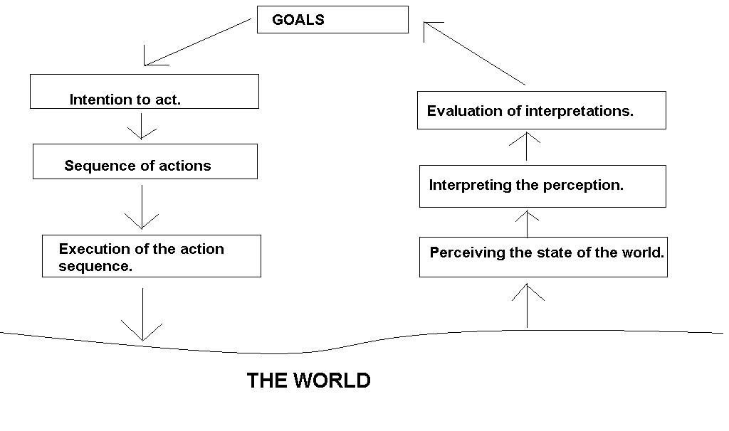
A Graphical Representation of the Software Testing Life Cycle
A you can see in the diagram below, errors can be introduced into the testing life cycle at multiple points. An error that would be introduced during the requirements specification could be an error of omission, while errors in the design, coding and fault resolution stages are more likely to be errors of commission.

Click to enlarge

Test Cases
Theory In order to craft a well constructed test case we must define a test scenario from entry to exit. This involves us understanding the purpose of the test as well as any preconditions and inputs which are involved in the test. The expected outputs are equally important as we must have a baseline to compare the results of the test to, in order to determine if they have passed or not. The postconditions are also important to be certain that the test is a complete success. Test cases must be tracked through the software life-cycle for traceability purposes and must also have a well defined reason for being. Precondition: something that must be true before the test case is executed Postcondition: some condition that must be true after the test case has executed.	Test Case Template Test Case ID Purpose Preconditions Inputs Expected Outputs Postconditions Execution History Date Result Version Run By Pass/Fail
Test Case Design "A test case is a set of instructions designed to uncover a particular type of error or defect in the software system by inducing failure."

What a Venn Diagram Can Tell Us
In the Venn Diagram we see two circles, one labelled A and the other B. Let's assume that circle A refers to the specified or expected behavior of an application, while circle B refers to the observed behavior of the same application. The intersection of A and B is where the requirements meet the programmed behavior. The portions of the circle in A which are not included in the intersection are requirements which have yet to be programmed and can be considered errors of omission. The areas of circle B which are not included in the intersection are equally a problem as they represent waisted effort on the part of the programmers since they have implemented functionality which has not been specified.


Testing Objectives
According to the Software Engineering Body of Knowledge (SWEBOK), the objectives of testing are the following:

 - Acceptance /  Qualification
 - Installation
 - Alpha & Beta
 - Conformance / Functional / Correctness
 - Reliability
 - Regression
 - Performance
 - Stress
 - Back to back
 - Recovery
 - Configuration
 - Usability

Structural Versus Functional Testing
Structural testing is used to create test cases based on the implemented code base, while functional testing focuses on testing the system from users point of view with absolutely no knowledge of how any of the functionality is implemented in code. Structural testing relies heavily on graph theory while functional testing relies more so on intuition and clearly stated functional requirements.

Types of Testing
Structural Testing	Functional Testing
Unit testing	Boundary value testing
Integration testing	Equivalence class testing
System testing	Truth table testing

White-Box Testing

This simply refers to testing methods which look "under the hood". The system is tested from the inside by verifying code, rather than testing by simply observing outputs.

Black-Box Testing

This type of testing is commonplace in the field of control systems. A black-box test is a test where the output of some input is observed for any errors. Thus this is a type of functional testing where we are really trying to verify if the system performs as expected for a given range of inputs. We have a concept of the expected output for each input and are making sure that it always corresponds. An example of black-box testing is system testing, acceptance testing, etc...

Unit Testing
The purpose of a unit test is to test a small subset or component of code in order to make sure it performs as expected. Unit testing occurs throughout the coding process, ideally before any code is even written. Test driven development (TDD) is the practice of writing unit tests before writing the code necessary to pass the tests. This offers the programmer the advantage of conceiving the code they intend to write before actually writing it. I know this may sound silly but it's actually extremely helpful. Once you have written a test case for some code, you have actually already began writing the code that you need to pass the test. I am an advocate of this type of testing and would recommend TDD to programmers with any amount of coding experience.

Integration Testing
Integration testing is similar to unit testing although this time the snippets of code being tested are not as simple. The goal with integration testing is to see how all of the moving parts fit together. Thus the integration test case's primary goal is to validate the interactions between components. Note that the components should have all been tested previously within independent unit tests.

System Testing
This is a higher level of testing than either the unit or integration tests. This type of testing is almost analogous to user acceptance testing. System testing is done at the system boundary level and it's primary goal is to evaluate the functionality of the system in terms of it's expected performance during it's intended use.

Regression Testing
Regression testing is used to ensure that newly written code is compatible with previously written code. The way this compatibility is measured is by running previously written tests on the newly expanded code base ensuring that no new bugs have been introduced into the system as the result of the additional code. Naturally there are limits to testing and every test can't possible be re-run every time the code has been updated, although it is expected that a sub-set of the tests which passed previously should be re-run.

The Law of Conservation of Bugs

"The number of bugs remaining in a system is proportional to the number of bugs already fixed."

Key Issues in Testing
 - The oracle problem
 - Limitations of testing
 - The problem of infeasible paths
 - Test selection criteria / Test adequacy criteria
 - Test effectiveness / Objectives for testing

The Oracle Problem
The oracle problem starts with a tale of 100 blue eyed people on an island and ends with them all being dead 100 days later. To summarize the story, everyone on the island does not know their own eye color nor can anyone else tell them. Everyone knows what color eyes everyone else has though, since they can all see. One day an oracle shows up on the island and tells everyone that some people have blue eyes. This is bad news because if you find out that you have blue eyes you must kill yourself alone at midnight. To make a long story short, everyone looks around and sees tons of other people with blue eyes thinking that they themselves don't. 100 days later everyone realizes that no one else has killed themselves meaning that they must be the ones with the blue eyes and so the tale comes to an end. On the surface this problem was not easy to relate to software testing and so I started a post at StackOverflow. Here is a quote from the post with the best explanation I got regarding the problem as it relates to testing. "I don't consider it (the oracle problem) a very good analogy, but the idea is that you can test a piece of software against something, some standard, to see if it gives the correct answer. The standard might be another piece of software, or the same software in a previous run, or theoretical results, or whatever. But how do we know the standard is correct? It would be really good to have a standard which is correct, and which everyone knows is correct, and which everyone knows everyone knows is correct, and so on." I think that this response is self explanatory once you've understood the oracle problem.

Limitations of Testing
Since everything has it's limits in life why shouldn't testing. Some programming problems have an infinite number of solutions and so it would be impossible to test every single possible outcome within a reasonable amount of time. Take any piece of code with an infinite loop and try to figure out how you could test every possible outcome (without running out of time first, possibly on your life). Combinatorial explosion is another instance where testing can get out of control, say 4 inputs exist with 5 possible values, 4⁵ combinations exist.

The Problem of Infeasible Paths
Not every line of code is necessarily reachable. Such paths are referred to infeasible and represent another limitation of testing. A basic example of this would be a line of code which could never be reached because of some Boolean condition in an IF statement which would never become true.


Functional Testing

---

Boundary Value Testing
Any computer program can be considered to be a mathematical function with values mapping from domain to the range. As an example, consider the input of the program to be it's domain and the range of the program to be it's output. While conventionally in boundary value testing an emphasis is placed on the input values, knowing what the expected output should be is an excellent way to squeeze more value out of the tests. Boundary value testing is an excellent way of getting rid of the pesky "off by 1" errors loops are prone to, it's also good way to uncover errors that exist at the extreme values of inputs.

How to Determine the Boundaries
A simple formula is available for us to come up with the boundaries of a certain variable. We will always define the following five values to be tested for each variable of interest:

Boundary values on a graph

Value	Denoted as
Minimum value	min
Just above minimum value	min+
Nominal value	nom
Just below maximum value	max-
Maximum value	max

The single fault assumption, from reliability theory, provides a critical enhancement to the process of boundary value analysis by proposing that rarely will a failure be the result of the simultaneous occurrence of more than one fault. This allows us to restrict the number of test cases necessary by holding all but one variables at their nominal values while testing the five possible values for a second variable. For some clarification here I'll list the set of test cases that would be needed to test two input variables, a and b.

set of test cases T = {<A_nom, B_min>, <A_nom, B_min+>, <A_nom, B_nom>, <A_nom, B_max->,
<A_nom, B_max>, <A_min, B_nom>, <A_min+, B_nom>, <A_max-, B_nom>, <A_max, B_nom>}

Using our math skills we can come up with a general equation for the number of test cases needed to conduct boundary value testing for any number of variables.

Y = the number of variables
Total number of unique test cases = (4 x Y) + 1

# of variables	Equation	# Test Cases
2	(4 x 2) + 1	9
3	(4 x 3) + 1	13
10	(4 x 10) + 1	41

As you can see the number of test cases rises linearly with the number of variables and so it is recommended to use automated tools to conduct this task most efficiently. Here is a link to a list of open source Java testing tools, some of which can be used to conduct boundary value testing in an automated fashion.

When no clear bounds exist for a variable we must artificially impose bounds on the variable.Although theoretically this seems unfair practically it isn't. Your computer can only perform calculations on a number of a finite size thus it makes sense to make a cap somewhere. Sometimes boundary value testing doesn't make as much sense, especially when it comes to Boolean variables thus it's use is limited in it's ability to provide value to the testing of an application. Boundary value testing works best when the program that it's testing is a function of many independent physical quantities. To put this statement into context, suppose we were testing a program that tests whether a date is valid. According to the above formula for formulating the test cases it is clear that the mechanically formed tests would capture the end of month and end of year date faults but it might not capture all of the leap year faults. When dealing with physical quantities the bounds are much more important, like length, height, speed, force. This is when boundary value testing is most appropriate.

Robustness Testing
Robustness testing is a small improvement over boundary value testing. If you noticed in boundary value testing we only approached the extreme valid numbers of a function, but never exceeded them. This is the value that robustness testing brings to the table. We'll add two more test cases to every variable to capture the programs behavior as it exceeds the upper and lower permissible bounds.

Value	Denoted as
Just below minimum value	min-
Minimum value	min
Just above minimum value	min+
Nominal value	nom
Just below maximum value	max-
Maximum value	max
Just above maximum value	max+

 This type of testing directs your attention towards exception handling.

Worst-Case Testing
In worst-case testing we push the envelope even further by introducing even more test cases. This time we revert back to the original five values for each variable as we had in boundary value testing, only this time we take the Cartesian product of the five test cases per variable, resulting in 5ⁿ test cases in total. We've discarded the single fault reliability theory in this case and augmented the number of test cases considerably. If you want to take worst-case testing even further you could combine it with robustness testing and up your number of test cases to 7ⁿ.

Special Value Testing
This is the most intuitive of all of the testing methods we've discussed so far as it relies on the intuition of the programmer to devise clever test to challenge the "soft spots" in the program. The challenge in promoting this type of testing is that it's outcome is largely dependent on the abilities of the programmer, which can be another potential source of error. Since the other tests we looked at don't encapsulate domain specific knowledge that the programmers may have, special testing can often be very effective at isolating problems in code.

Equivalence Class Testing
Since boundary value testing doesn't satisfy our need for complete without redundancy we need something a little bit more powerful to help us.Boundary value testing can be thought of as forming the lines around a box, whereas equivalence class testing takes the same box yet breaks it apart into puzzle pieces that form the whole. The value of breaking the box into pieces is that each of piece can be thought of a set of values with something in common. This is a powerful notion as it allows us to further divide the square into logical components which form a set of data which can be used for testing. Thus by taking one element from each set (puzzle piece) we can form a more comprehensive set of test that eliminate redundancies and provides a sense of completeness, since an element from each puzzle piece is tested, and all of the puzzle pieces together form the entire square. By choosing your equivalence classes wisely you can reduce the number of test cases needed while improving the quality of them greatly.

Weak Normal Equivalence Class Testing
In weak normal equivalence class testing we only use one value from each equivalence class in a test case. By using one value only from each equivalence class we are once again employing the single fault assumption. The number of test cases generated using this form is testing is always equivalent to the number of equivalent classes defined.

Strong Normal Equivalence Class Testing
In strong normal equivalence class testing we use the multiple fault assumption in lieu of the single fault assumption. This provides a sense of completeness in our testing since we take the Cartesian product of all of equivalence classes. The result of taking the cross product will yield a result similar to that which a truth table would produce.

Weak Robust Equivalence Class Testing
Since the name (weak and robust) is counter intuitive we'll break it down make some sense of it. The robust part, as before, alludes to the consideration of invalid values, while the weak part refers back to the single fault assumption. Thus to craft our test cases for the valid inputs we will use one value from each valid  equivalence class, just as we did in the weak normal equivalence class testing. For the invalid inputs we will associate one invalid input to every equivalence class (note the single fault assumption). Weak robust equivalence class testing can often become awkward in modern strongly typed languages. It was a much more popular form of testing historically when languages like COBOL and FORTRAN dominated the scene. In fact, strongly typed languages were developed to address the faults often uncovered by weak robust equivalence class testing.

Strong Robust Equivalence Class Testing
This time the name is not as confusing as it is redundant. As usual the robust part of the title refers to the consideration of invalid inputs, while the strong part implies the multiple fault assumption. This time we derive our test cases from the Cartesian product of each element from the equivalent classes.

Decision Table-Based Testing
Of all the functional testing methods seen so far, decision tables offer the most complete form of testing since they are the most rigorous. Two types of decision tables exist, limited entry decision tables and extended entry decision tables. The difference between the two is the type of conditions that a value can take. In a limited entry decision table only binary conditions can apply, while in an extended entry decision table three or more conditions may apply. To identify the test cases from a decision table we interpret the conditions as inputs to our program and actions as the outputs. Recall that in a binary decision table the total number of rows necessary is 2ⁿ, where n is the number of variables being tested. So two variables with binary conditions yields a truth table with 4 rows and 2 columns and three variables yields a table with 8 rows and 3 columns. Use decision table testing for programs that have a lot of decisions being made.


Here's a little graphical review for you to crystallize the trends of effort and sophistication involved in the functional testing methods seen.

How to Determine What Type of Functional Testing is Most Appropriate

C1	Variables (P, physical; L, logical)	P	P	P	P	P	L	L	L	L	L
C2	Independent variables?	Y	Y	Y	Y	N	Y	Y	Y	Y	N
C3	Single fault assumption?	Y	Y	N	N	-	Y	Y	N	N	-
C4	Exception handling?	Y	N	Y	N	-	Y	N	Y	N	-
A1	Boundary Value Analysis		X
A2	Robustness Testing	X
A3	Worst-Case Testing				X
A4	Robust Worst-Case			X
A5	Weak Robust Equivalence Class	X		X			X		X
A6	Weak Normal Equivalence Class	X	X				X	X
A7	Strong Normal Equivalence Class			X	X	X			X	X	X
A8	Decision Table					X					X

Structural Testing

---

The key trait of structural testing is that it is based on the source code of the application instead of on it's specifications. Since structural testing is based on the implementation the most basic step we can take to define a program mathematically is to create a program graph.


Program Graph

Click to enlarge

A program graph is a directed graph representing a program whereby the nodes in the graph represent statement fragments while the edges represent the control flow. So in the graph depicted on the right side we have two variables declared immediately, i and j, followed by a control statement which leads to two different states. From there we proceed to exit the control statement and head to the final statement where the value of j is returned. Loops in code can also be easily graphed using the same principles which we have applied here. A loop will always contain a control statement that will verify whether or not the loop should continue, and from there you might either return into the loop or head towards another state unrelated to the loop. No matter what type of control flow statement you face rest assured that the same principles apply in graphing them. The only thing you need pay attention to is at which point in the code the decision making occurs. Note that normally in a Program Graph you would not label the nodes with actual statements from the program but more likely a statement number (or line number, when only one statement appears on each line). Here is a tiny sample of how to model a For-loop.

Click to enlarge

DD-Paths

Click to enlarge

Decision to Decision Paths are the most widely used form of structural testing, created by Miller in 1977. What distinguishes DD-Path graphs from Program Graphs is the level of granularity with which the program is decomposed. In a program graph every statement within the program is given it's own node. In a DD-Path graph only nodes that lead to decisions (control flow) are given their own nodes. Thus we can now appreciate the original description provided by Miller: a path begins with the "outway" of a decision statement and ends with the "inway" of the next decision statement. In order to demonstrate this concept I've converted the above Program Graph into a DD-Paths graph. Note that I've re-labelled the vertices with numbers representing the statement number based on the order of the statements in the Program Graph. This follows a more conventional style of labeling nodes seen in most examples and texts. In the DD-Paths graph illustrated on the right there are two unique (linearly independent) paths that can be enumerated, 3,4,6,7 and 3,5,6,7.

Formal Definition of DD-Paths
A DD-Path is a sequence of nodes in a program graph such that:
  Case 1: It consists of a single node with indegree = 0.
  Case 2: It consists of a single node with outdegree = 0.
  Case 3: It consists of a single node with indegree >= 2 or outdegree >= 2.
  Case 4: It consists of a single node with indegree = 1 and outdegree = 1.
  Case 5: It is a maximal chain of length >= 1.

This formal definition on the surface is a little hard to appreciate so we'll decompose it and find out what it means. Case 1 refers to the fact that every graph must have a starting node, which does not have any edges directed in towards it. Case 2 establishes that the graph must have a terminal node, which does not have any edges directed away from it. Case 3 states that a complex node must not be contained within more than one DD-Path. Case 4 is needed to enforce against a short path while also preserving the one-fragment, one-DD-path  principle. Case 5 is the case in which a DD-Path is the is a single-entry and single-exit chain. The maximal part of case 5 is used to determine the final node of a normal chain.

So What is a DD-Path Graph Good For?
The insight that DD-Path graphs bring to programmers is the ability to quantify testing coverage precisely. This is rather important when attempting to determine the extent to which code has been tested, and as we've noted earlier there are limitations to testing (Hint: testing loops). According to E.F. Miller (1991), when DD-Path coverage  is attained by a set of test cases, roughly 85% of all faults are revealed. This is a very significant statistic and should act as motivation for every software engineer to enforce even the most basic testing methods as the benefits far outweigh the effort.

McCabe's Basis Path Method

V(G) = 10 - 7 + 2(1) = 5

In the 1970's, Thomas McCabe applied some breakthroughs in graph theory related to the cyclomatic number of a strongly connected graph to computer science in order to determine the number of linearly independent paths in the graph. Thus the cyclomatic complexity of a graph is equal to the number of linearly independent paths in the graph. The graph depicted on the right is a classic example cited in many texts. Since the graph on the right is not strongly connected we will need to add an edge from node G back to A in order to apply the cyclomatic complexity (denoted V(G)) calculation.

Cyclomatic complexity of a weakly connected graph:
V(G) = e - n + 2p
e is the number of edges

V(G) = 11 - 7 + 1 = 5

n is the number of nodes
p is the number of connected regions

Cyclomatic complexity of a strongly connected graph:

V(G) = e - n + p

e is the number of edges

n is the number of nodes

p is the number of connected regions

As we can see the cyclomatic complexity for both the strongly and weakly connected graphs are equivalent. Here is a list of all 5 linearly independent paths in the graphs on the right.

Path 1: A, B, C, B, C, G 

Path 2: A, B, C, G

Path 3: A, B, E, F, F

Path 4: A, D, E, F, G

Path 5: A, D, F, G

Computing Minimum Number of Test Cases
In order to calculate the minimum number of test cases needed to traverse all statements, branches, simple-paths or loops in a graph we'll need to use the prime decomposition theorem. It states that any graph can be decomposed into a unique prime representation. This is good news for us because it's basically going to give us some shorthand to account for complexities in our graphs. Once we've found the prime decomposition of the graph we will use a slightly different method to calculate the minimum number of test cases based on our traversal objectives.

Click to enlarge.

How to Create a Prime Graph
The trick as I mentioned earlier is that we will be creating some short hand for the types of statement that we can encounter in programming which would alter the complexity of our graph. Here is legend that refers to the programming construct and the related shorthand notation.

Perhaps one of the best ways to learn how to decompose a graph will be to learn from an example. On the left hand side of the diagram below you will notice the corresponding control flow graph, while on the right hand side you will find the associated prime decomposition.

So, after you've decomposed your graph and have found it's prime representation you can move on to figuring out what the minimum number of test cases will be. Depending on the strength of the type of testing you choose you will assign different values to each prime in the graph. We will then take the maximum value of the primes and add 1 to if to determine the minimum number of test cases. So the formula is m(F) = Max + 1, written quite informally here where the max is the highest value assumed by any prime in your decomposition graph according the charts below.

Dataflow Testing
This is a form of structural testing that focuses on the points at which variables are assigned values as well as the points at which those variables are referenced. This is in contrast to DD-Paths testing where we focus on the control flow of the program instead of the variable assignments. The types of errors that become most visible in dataflow testing are known as define/reference anomalies:

  - A variable that has been defined but never used (referenced)
  - A variable that is used before it has been defined
  - A variable that has been defined twice before it has been used

Define/Use Testing
Define/Use testing focuses on the lifetime of a variable throughout your program. We construct a program graph in a similar way as we defined earlier only this time the nodes of the graph represent events associated with variables only. The events associated with variables are broken down into two categories, definitions and uses, hence the title.

Definitions
DEF(v, n) - variable v at node n has changed in value

Formal definition: node n element of G(P), is a defining node for the variable v element of V, iif the variable v is defined at the statement fragment corresponding to node n. The following is a list of statements which are all considered to be examples of defining nodes:
- Input statements
- Assignment statements
- Loop control statements
- Procedure calls

Uses
USE(v, n)  - variable v at node n has not changed in value

Formal definition: node n element of G(P), is a usage node of the variable v element of V, iif the variable v is used at the statement fragment corresponding to the node n. The following is a list of statements which are all considered to be examples of usage nodes:
- Output statements
- Assignment statements
- Conditional statements
- Loop control statements
- Procedure calls

**The most important notion to remember about Define/Use testing is that the value of the variable changes when it is defined and does not when it is used.

One last subtlety about def/use testing before we wrap things up.

Usage nodes can be further decomposed into predicate uses and computational uses. A predicate use, denoted P-USE(v, n), is defined as the usage of a variable v at node n, such that the corresponding statement fragment is a predicate. A computational use, denoted C-USE(v, n), is defined as the usage of variable v at node n, such that the corresponding statement fragment is a computational use. Take note that the node n will have an outdegree greater than or equal to 2 in the case of a P-USE. In the case of a C-USE the outdegree of node n will always be equal to 1.

Now that we know how to define a node as being either a DEF or USE we can now proceed to the formal definition of a definition-use path, denoted du-path.

Definition of a DU-Path
a du-path with respect to variable v element of V is a path in PATHS(P) such that there exists define and usage nodes, DEF(v, m) and USE(v, n) where m and n are the initial and final nodes of the path.

Definition of a DC-Path
a definition clear path, denoted dc-path, with respect to variable v element of V is a path in PATHS(P) such that DEF(v, m) and USE(v, n) are the initial and final nodes of the graph respectively, additionally no other definition node exists for variable v other than DEF(v, m). This formal definition is just saying that for a single variable, the dc-path only contains a single node at which the respective variable is defined.

What this all boils down to is a single piece of advice... du-paths which are not definition clear are potential points of error in your code.

Test Coverage Metrics for DU-Paths: Rapps & Weyuker Dataflow Metrics
Now that we have defined all of the flavors of du-paths we can come up with some metrics to gauge our test coverage. The five metrics we will use are: All-Defs, All-Uses, All-DU-Paths, All-P-Uses/Some-C-Uses and All-C-Uses/Some-P-Uses.

All-Defs
The set of paths T in program graph G(P) of program P satisfies the all-defs criteria iif for every variable v element of V, T contains definition-clear paths from every defining node of v to a use of v.

Rapps-Weyuker hierarchy of dataflow coverage metrics

All-Uses
The set of paths T in program graph G(P) of program P satisfies the all-uses criteria iif for every variable v element of V, T contains definition clear paths from every defining node of v to a use of v, as well as to the successor node of each USE(v, n). This is the union of all C-USES and P-USES.

All-DU-Paths
The set of paths T in program graph G(P) of program P satisfies the All-DU-Paths criteria iif for every variable v element of V, T contains definition clear paths from every defining node of v to every use of v, and to the successor node of each USE(v, n), and that these paths are either single-loop traversals or cycle free.


All-P-Uses/Some-C-Uses
The set of paths T in program graph G(P) of program P satisfies the All-P-Uses/Some-C-Uses criteria iif for every variable v element of V, T contains definition clear paths from every defining node of v to every p-use of v, and if a definition of v has no p-uses, there is a definition clear path path to at least one C-use.


All-C-Uses/Some-P-Uses
The set of paths T in a program graph G(P) of program P satisfies the All-C-Uses/Some-P-Uses criteria iif for every variable v elements of V, T contains definition clear paths from every defining node of v to every c-use of v, and if a definition of v has no c-uses, there is a definition clear path to at least one p-use.

Slice-Based Testing
A program slice is a set of program statements that contribute to the to the value of a for a variable at some point in the program. This perspective allows us to observe the behavior of a certain variable in isolation.

Formal definition: A slice S on the variable set V at statement n, denoted S(V, n), is the set of all program statements prior to node n that contribute to the values of variables in V at node n. Note that listing all of the program statements which contribute to the values of the variables in V can be a lot of work. To speed things up it is recommended to list the node numbers in the path which affect the values of the set of variables in V. This means that USE nodes are not included in the set, only DEF nodes are.


White-Box Testing Strategies Strength Ranking:

*Note, the more +'s the more strength

+            statement coverage

++          decision coverage

+++        condition coverage

++++      condition decision coverage

+++++    multiple condition coverage

++++++  path coverage (implicitly provides branch coverage)

Integration Testing

---

Functional Decomposition Tree

Decomposition-Based Integration
Integration testing occurs once all of the unit testing has been completed. In fact, it presupposes that all of the code has already been broken down into functional units and that independently each performs as expected. The goal of integration testing is to combine multiple code units into coherent workflows and test the interactions between the various components. With this in mind I'll introduce the concept of the functional decomposition tree. The functional decomposition tree is the basis for integration testing as it represents the structural relationship of the system with respect to it's components. The way to construct the functional decomposition tree is to create nodes with directed edges, where the nodes represent modules or units and the edges represent the relationships or calls between these units. There are three main methods that can be used to traverse the tree: top-down, bottom-up, sandwich and the big-bang.

Functional Decomposition-Based Integration Methods
Top-Down Integration
Traverse the tree from the top-down using a breadth-first approach, placing stubs where lower level units would normally be called. Stubs are throw away code fragments representing simulations of lower level units.The trick with the top-down approach is to gradually replace stubs with functional code. Suppose you have a unit with an outdegree of 5 and you replaced all of the stubs simultaneously, you could be creating a "small-bang".

Bottom-Up Integration
Traverse the tree from the bottom-up using drivers to simulate higher level modules making calls the lower levels. This is exactly the same thing we've done in top-down integration only now we're approaching the graph from the bottom up. The only difference here is that we use drivers instead of stubs. Drivers are throw away bits of code as well but in practice it has been shown that drivers require less effort to create than stubs. Additionally due to the fan-out nature of most code, less drivers will be required to be written, albeit they will likely grow in complexity which in itself is a caveat.

Sandwich Integration
This is a hybrid of the top-down and bottom-up methods where the tree is traversed simultaneously from both directions. This will result in you doing a big-bang on the various sub-trees, think of it as a depth-first approach to traversing the tree. The advantage here is that less drivers and stubs will be needed, however this convenience comes at the expense of reduced fault isolation.

Big-Bang
In this method you simply test the code as one giant unit. This method requires the least effort although it also offers the least visibility for fault isolation.

Formula to calculate the number of integration tests needed:

Sessions = nodes - leaves + edges

- For top-down integration,  nodes - 1 stubs are needed
- For bottom-up integration, nodes - leaves drivers are needed
*Note, a session is one set of tests for a specific configuration of code and stubs.


Call Graph Based Integration
Pairwise Integration
The goal of pairwise integration is to eliminate the need to develop stubs and drivers. Instead of using these throw away bits of code we resort to using the actual code in a more controller manner. We restrict a session to a pair of units in the call graph. The result of this restriction is that every edge on the call graph forms the basis for a test case. Thus the number of edges in the graph represents the number of test cases needed. The savings here is not in the number of test cases needed, as compared to the aforementioned decomposition-based integration methods, but rather in the reduced effort related to driver and stub development.


Neighborhood Integration
By taking pairwise integration one step further we arrive at neighborhood integration. This method borrows the notion of a neighbor from topology theory, where a neighbor is defined as a node separated from the node of interest by a certain radius, normally 1. Thus all of the nodes one away from the node of interest, immediate predecessors and successors, are deemed to be within the neighborhood. The advantage of using this method is that the number of sessions can be greatly reduced, as compared to pairwise integration. Additionally there is a reduction in the number of drivers and stubs needed but we're essentially forming sandwiches, which as we saw have their own problems. To compute the number of neighborhoods on a call graph we use the following formula:

Neighborhoods = interior nodes + source nodes
This formula  can also be rewritten as
Neighborhoods = nodes - sink nodes
*Note, interior nodes have an indegree and outdegree >= 1, and source nodes are the roots of the tree.


The advantage of employing call graph based integration methods over functional decomposition trees is that we are moving away from a purely structural basis to a behavioral basis. These techniques also reduce the need for driver and stub development. The largest issue with graph-based integration is that fault isolation is reduced since we are dealing with compounded units of code. This can be especially troublesome when multiple units (nodes) all converge to a common node. Errors introduced at that point will likely require some code modifications in order to better isolate the fault, and re-testing of previously tested components becomes necessary.

Path-Based Integration
MM-Path
The idea behind path based integration is to trace a path through the source code as it executes resulting in a graph similar to a DD-Graph although this time we don't use decisions as a means to trace the control flow but rather use the invocations of units as edges on the graph. Notice again how we assume that the unit testing has been completed before moving on to this level of testing. MM-Paths are a hybrid of structural and functional testing, with the greatest advantage being that path based testing is closely related to system behavior.  Thus in order for us to construct an MM-Path we'll use the following definitions to guide us.

Source Node
A source node in a program is a statement fragment at which program executions begins or resumes.

Sink Node
A sink node is a statement fragment at which program execution terminates, or at which control is passed to another unit.

Module Execution Path
A module execution path is a sequence of statements that begins with a source node and ends with a sink node, without any intervening sink nodes (remember integration testing is presumed to be compete).

Message
A message is a mechanism by which one unit transfers control to another unit. Examples of messages are: method invocations, procedure calls and function references.

MM-Path
An MM-Path is a sequence of module execution paths and messages.

"A program path is a sequence of DD-Paths while a MM-Paths are a sequence of module execution paths."

Guidelines for Determining the Length of an MM-Path
Two main indicators should be used to restrict the length of an MM-Path. The first is message quiescence and the second is data quiescence. Message quiescence occurs when a unit that doesn't send any messages is reached. Data quiescence occurs when a a sequence of processing culminates in the creation of data that is not immediately used.

Analyzing the Complexity of an MM-Path
The way to analyze the complexity of an MM-Path is to calculate it's cyclomatic complexity. Recall V(G) = e - n + 2p, but in this case p is always equal to 1.

System Testing

---

The focus of this type of testing is at a very high level, in contrast to functional and structural testing. The goal of system testing is to verify whether or not the system is doing what it is supposed to be doing. The basis from which a functional test is derived is a behavioral or functional specification.  In order to determine whether or not the system is behaving as expected, tests must be based upon workflows, use cases, etc... Notice how we are drawing inspiration from elements which lie at the boundary of the system. The basic construct that is used to build system tests is a thread. In the simplest terms a thread encapsulates the idea of one user level system goal. There is some controversy over the exact description of a thread and I'll do my best to describe it in an intuitive way, based on what we already know about testing. Unit testing tests individual functions, while integration testing focuses on interactions between units and system testing examines interactions among atomic system functions.

Atomic System Function (ASF)

An atomic system function is a unit of code, which should have undergone unit testing by the time you've gotten to system testing. ASF's are the building blocks from which system tests are derived. Unit level ASF's are the components which are used to construct DD-Paths with, while integration level ASF's are used to construct MM-Paths. Continuing along this trend we can restate our definition of a thread as a series of MM-Paths. Generally, an ASF is an action that is observed at the system level in terms of port input and output events (system boundaries).

The Basic Concepts Used for Requirements Specifications
Since we now know that structural testing is based on verifying whether or not the system has met the user's requirements, a natural place to turn for testing inspiration is the requirements. It can often be difficult to determine how all the moving pieces inside the software system are supposed to interact and that is where some good design and architecture documents provide value. The requirements for a system can generally be broken down into the following five views: Data,  Actions, Devices, Events, Threads.

Data
When analyzing the data associated with a system attention is paid to how the data will be used, created and manipulated. A typical way of modeling the data view of a system is using an Entity/Relationship  diagram. The focus of the E/R model is to label data structures and provide insights on the data's relationship with other entities.


Actions
Action based modeling is still used commonly today, although it was even more popular when imperative programming was the "new kid on the block". Actions have inputs and outputs represented by either data or port events. The I/O view of actions is the basis of functional testing while the decomposition of actions is the basis for structural testing. Actions are analogous to functions, methods, calls, processes, tasks, etc...

Devices
Computer systems have a variety of ports used by external devices for communication. Although a port usually reminds us of a plugging in some external device, we can abstract this notion a step further by considering a port simply as a vehicle for input and output. This abstraction is useful in testing because it allows us to draw the focus away from the port devices and closer towards the logical relationship the ports have with the system.

Events
An event can be thought of as the translation of a physical event to a logical event occurring on a port device. A keystroke is an example of an event, as is updating a display. That being said we can see that an event has both data and action like properties.

Threads

A typical use of the system, in software terms, can be described as a  thread. A thread is a sequence of source instructions executed in conjunction with the servicing of a user's goal. Typically, a thread will be composed of calls to multiple classes or interfaces (MM-Paths). A thread is the highest level construct used in integration testing, but the smallest construct considered in system testing. One of the best ways to represent a thread is by using a finite state machine.

Thread Testing
The way to go about testing threads isn't revolutionary, although it does require some thought. We will use port input and output events as the road map for creating graphs, which will be conjunctions of finite state machine representing threads. In this view, should we find it necessary test any particular thread more carefully, we would basically be conducting integration testing. Going even further we could then resort to unit testing to get to the root of any bug. We will encounter the issues with system testing graphs as we did with unit and integration testing in regards to path explosion. This forces us to choose our test paths wisely by taking advantage of the knowledge the directed graphs provide us with.

Finding Threads
The general strategy for finding threads is by tracing input and output events on a system level finite state machine. As we mentioned previously, a use-case or some other high level sequence of interactions with system are used to create the context for the state machine. It is recommended to create the state machine such that transitions correspond to port input events, while port output events are represented by actions on transitions.

Structural Strategies for Thread Testing
Since we are using directed graphs to represent the interactions of threads we can reuse the same test coverage metrics we discovered in unit testing, namely node and edge coverage. Node coverage at the system level is equivalent to statement coverage at the unit level. Node coverage is the minimum a tester can do, although the recommended approach is to use edge coverage. Edge coverage at the system level has the added benefit of guaranteeing port event coverage as well.

System testing becomes a little bit more complicated when we don't have a behavioral model for the system to be tested. This will require us to find inspiration within three of the aforementioned basis concepts: ports, events and data.

Event-Based Thread Testing
We begin thinking about event based thread testing by considering port input events. Within the realm of port input events the following five coverage metrics are introduced:

PI1: Each port input event occurs
PI2: Common sequences of port input events occur
PI3: Each port input event occurs in every relevant data context
PI4: For a given context, all inappropriate input events occur
PI5: For a given context, all possible input events occur

The PI1 metric is regarded as the bare minimum and is often inadequate for proper testing.

PI2 coverage is the most common because it emanates from the most intuitive view, the normal use of the system. Within the scope of defining normal use of the system is may not necessarily be trivial to identify all commons sequences of port input events.

PI3 coverage like PI4 and PI5 are context specific metrics. We will define a context as a point of event quiescence. Event quiescence is the point at which some event terminates, an example of this is a screen popping up letting the user know the supplied username and password combination is invalid. These points in an event driven system will normally correspond to responses provided by the system to user requests (which are also events).

So getting back to the definition of PI3 coverage, the focus in this scenario is on developing test cases that are based on events that have logical meanings determined by the context in which they occur. Consider an example at an ATM machine, where the buttons on the sides of the screens take on different actions depending on what point in the transaction sequence you are at. The thing to remember about PI3 coverage is that is driven by an event within each context.

PI4 and PI5 coverages are opposite of one another. The both start with a context though and seek to describe relevant events. PI4 begins with a context and seeks to wreak havoc on the system by supplying strictly invalid inputs, while PI5 attempts to only provide valid inputs. The PI4 metric is normally used on more of a casual hacking basis, so as to uncover weaknesses in the system. PI4 and PI5 are both effective methods at testing a system although some interesting questions arise when we begin to think about breaking the system. A Venn diagram could really help out here, let's imagine one. The circle on the left represents all of the inputs a system is designed to handle. The circle on the right contains every other possible input which has not been defined in the system specification. The union of the two circles represents the inputs which have been specified by the system that are invalid. Now the question is, how do we quantify what the remainder of invalid inputs that exist in the circle on the right? That is challenge in testing with PI4. PI5 testing is much more straight-forward since the requirements should provide all of the information needed to determine what the valid inputs exist.

Port Coverage Metrics
 Another metric that can be used to gauge the graph coverage is port coverage:


PO1: Each port output event occurs
PO2: Each port output event occurs for each cause

PO1 coverage is acceptable minimum and is extremely useful when a system has a large variety of output messages when errors occur. PO2 coverage is a worthy goal however it can sometime be difficult to quantify. PO2 coverage focuses on threads that interact in response to a port output event, note that output events are usually caused by very few inputs.

Port-Based Thread Testing
Port-based thread testing is useful when used in conjunction with event based testing. The strategy here is to determine which events can occur at each port. Once the list has been compiled we seek threads that will test each possible event at a port with port input and output. Event-based testing exposes the many to one relationship between events and ports. Port-based testing looks at the relationship from the opposite perspective, identifying the many to one relationship between ports and events. This type of testing is especially useful for systems when third party suppliers provide port devices.

Data-Based Thread Testing
Systems that are event based are not good candidates for data-based testing, usually. Data driven systems on the other hand oddly enough lend themselves well to data-based thread testing. Since data based system will often have requirements stipulated in terms of the modification of some data, these actions form a natural basis to identify threads. For example, suppose we were looking at a system designed to keep track of video rentals. Much of the systems functionality would be prescribed in terms of data transactions, like create client accounts, rent movies, return movies, etc... The best way to analyze the data of a system is to look at the E/R diagrams. The relationships in the E/R diagrams are particularly useful to notice since system level threads are usually the ones responsible for populating the relevant data for each entity. At the system level it is more likely that we would encounter threads which are responsible for maintaining data for a single entity.

DM1: Exercise the cardinality of each relationship
DM2: Exercise the participation of every relationship
DM3: Exercise the functional dependencies among relationships

The cardinality of a relationship refers to the following four types of relationships: one-to-one, one-to-many, many-to-one and many-to-many. Each one of these possibilities can be seen as a thread from a testing perspective.

Participation relates to the the level of participation of each entity within a relationship. For instance, in a many-to-many scenario each entity would need to be observed to ensure that it properly fulfilled it's relationship specifications. These points of observation could easily be turned into system level testing threads.

Functional dependencies are stringent logical relationship constrains that are placed upon entities. These dependencies naturally become converted to threads which are testable.

Operational Profiles
Zipf's law states that 80% of a systems activity occurs within 20% of the space. This law manifests itself in software as the principle of locality of reference. The implication of this law on testing is that some threads will be traversed more often than others. Thus if we were to evaluate the reliability of the system, failures which occur in popular threads would cause the majority of the problems. The intuition here is that we if we focus on testing threads that occur more often we could potentially increase the reliability of the system immensely. Less tested threads which still may contain faults produce less errors overall since those threads are not executed as often. An operational profile is the concept of determining the execution frequencies of various threads, and then using this information in deciding which threads to test. One of the best ways to keep tabs on which threads occur most often is to assign weights to edges in the finite state machines representing how often that edge will be traversed. Using this method it is easy to determine what the probability that a given thread will be executed, simply multiply all of the probabilities along the way.

Progression Testing Versus Regression Testing
Regression testing is used to verify that any new functionality that has been added to a system has not compromised any previously functioning components from earlier builds. As the number of builds increases, the number of tests re-run on previously built components becomes non-trivial. Progression testing is that act of conducting tests on newly built components. Naturally we expect the number of failures to be much higher for the progression tests than the regression tests. So in order to be certain that the newly written code is bug free we must devise a plan that will allow us to easily isolate faults in the code. The best way to do this is create small threads for starters that can only fail in a few ways. After we have sufficiently tested a small thread we can integrate it into a larger thread, thus furthering our testing. We would use the opposite strategy for regression testing, having longer threads with more potential sources of error since we are less concerned with fault isolation in regression tests. As a general rule of thumb we can say that "good" regression testing utilizes threads with low operational frequency while progression testing threads should focus on high operational frequency threads.

Software Reliability Engineering (SRE)

---

Classical Definition of Reliability
Software reliability is the probability that a system will operate without failure under given environmental conditions for a specified period of time. Reliability is measured over execution time so that it more accurately reflects system usage. Software Reliability goes hand-in-hand with software verification.

Essential Components of Software Reliability Engineering

• Establish reliability goals
• Develop operational profile
• Plan and execute tests
• Use test results to drive decisions

Approaches to Achieve Reliable Software Systems
Fault Prevention
To avoid, by construction, fault occurrences.

Fault Removal
To detect, by verification and validation, the existence of faults and eliminate them.

Fault Tolerance
To provide, by redundancy, service complying with the specification in spite of faults having occurred or occurring.

Fail/Failure Forecasting
To estimate, by evaluation, the presence of faults and the occurrence and consequences of failures.

Software Reliability Models

Time-dependent

• Time between failures
• Failure count

Time-independent

• Fault seeding
• Equivalence classes

Time-dependent Reliability Models
Reliability Measures: MTTF, MTTR, MTBF


Mean Time To Failure (MTTF)
Total operating time dicided by the total nmber of faulures encountered (assuming the failure rate is constant)

Mean Time To Repair (MTTR)
Software component


Mean Time Between Failures
MTBF = MTTR + MTTF

Reliability Growth Models

• Basic Exponential model     - Assumes finite number of failures over infinite amount of time
• Logarithmic Poisson model - Assumes infinite number of failures

Parameters involved in reliability growth models:
1) λ = Failure intensity, i.e. how often failures occur per time unit.
2) τ =  Execution time, i.e. how long the program has been running.
3) μ = Mean failures experienced within a time interval.

Jelinski-Moranda Model
Assumptions:

• The software has N₀ faults at the beginning of the test
• Each of the faults is independent and all faults will cause a failure during testing
• The repair process is instantaneous and perfect, i.e., the time to remove the fault is negligible, new faults will not be introduced during fault removal.

Time-independent Reliability Models

Fault Seeding (Injection)
The definition of fault seeding is as follows. Fault seeding is the process of intentionally adding errors into a software program for the purpose of estimating the number of faults that are already contained within the system. What the definition doesn't tell you is how you can estimate how many faults still exist in the program. The number of faults estimated to be remaining in the system is a function of the programmers ability to discover the faults which have been intentionally introduced.


Let A represent the number of faults intentionally introduced
Let f be the number of failures that have occurred as a result of executing the flawed code
Let i be the number of failures which did not emanate from the newly introduced faults (All failures - f)
Finally let N - i represent the estimated number of faults remaining in the code


N / i = A / f, rearranging to solve for N we have N = A / (f * i)
finally we calculate N - i to get the estimated number of remaining faults in the system


Equivalence Classes
In order to derive an equivalence class in system testing you must create an operational profile for each thread. Once this profile has been created you should have a weight that refers to the likelihood that thread would be called during the execution life-cycle. Each path through the operational profile provides you with an equivalence class. Each path has a certain probability of execution which is obtained by multiplying the probabilities of each thread in the path.

Software Versus Hardware Reliability

Software Reliability	Hardware Reliability
Failures are primarily due to design faults. Repairs are made by modifying the design to make it robust against conditions that can trigger a failure.	Failures are caused by deficiencies in design, production and maintenance.
The is no wear-out phenomena. Software Errors occur without warning. “Old” code can exhibit an increasing failure rate as a function of errors induced while making upgrades.	Failures are due to wear or other energy-related phenomena. Sometimes a warning is available before a failure occurs.
There is no equivalent preventive maintenance for software.	Repairs can be made which would make the equipment more reliable through maintenance.
Reliability is not time dependent. Failures can occur when the logic path that contains an error is executed. Reliability growth is observed as errors are detected and corrected.	Reliability is time related. Failure rates can be decreasing, constant or increasing with respect to operating time.
External environment conditions do not affect software reliability. Internal environment conditions, such as insufficient memory or inappropriate clock speeds do affect software reliability.	Reliability is related to environmental conditions.
Reliability cannot be improved by redundancy, since this will simply replicate the same error. Reliability can be improved by diversity.	Reliability can usually be improved by redundancy.
Failure rates of software components are not predictable.	Failure rates of components are somewhat predictable according to known patterns.
Software interfaces are conceptual.	Hardware interfaces are visual.
Software design does not use standard components.	Hardware design uses standard components.

Model Checking and Formal Verification

---

Any verification using model-based techniques is only as good as the model of the system. As all other engineers must be embrace mathematics, software engineers should embrace formal methods.

Model Verification

Input	Output
formal model + property	Model Checking: True ; Counter Example

Testing Versus Model Checking

Testing	Formal Methods
Informal specification	Work on a model of the program
Cannot exhaustively test the system	Targets concurrent systems
Widely used technique in practice	Successful in hardware systems and communications protocols

Temporal Logic
The formulas can express fact about past, present and future states.


Classification of Temporal Properties
1) Safety:     properties state that nothing bad can happen
2) Liveness: properties state that something good will eventually happen
3) Fairness: properties state that every request is eventually granted




More to come soon....
Excellent Book on the topic: